Fundamentals of ANOVA

• ANOVA is unlike a t-test in that more than two groups are permitted
• Independent variable is categorical (e.g., year in school, experimental condition)
• The independent variable is often called a "factor".
• The values of the independent variable are called the "levels".
• Dependent variable is continuous
  
• Tests the null hypothesis that the means of two or more groups (specified by the different levels) are equal
  
• Alternative hypothesis is that at least one group differs significantly from one or more of the others
  
• Assumptions of ANOVA
  • Observations are independent of one another
    
  • The continuous dependent variable is distributed close to normal
    
  • The variance of the continuous dependent variable is roughly equal in all groups
    

Brief Discussion of How ANOVA Works (a longer discussion)

• ANOVA analyzes variance by separating it into two parts
  • Within-groups variability
    
  • Between-groups variability
• F statistic indicates whether the between-groups variability is significantly greater than the within-groups variability
  
• If the F statistic is significant (p < .05), at least one group mean is significantly different from one or more of the others
  
• A significant F statistic suggests that we reject the null hypothesis
  

Using SPSS to do single factor ANOVA

To set up an independent (between groups) one-way ANOVA you will need two columns of data, one for the idependent variable (a categorical variable which specifies which group each case belongs to) and one for the dependent variable (the thing you measured).

Go to the Analyze menu and select the submenu Compare Means. In this submenu you'll see several tests. The one that we're interested in today is One-way ANOVA.
After selecting One-way ANOVA you'll get a window that looks like this. Here you should select the variables that you are testing. Your "Dependent List" is your dependent variable (the continuous variable that you measured). Your "Factor" is the independent variable that assigns each subject to a group.
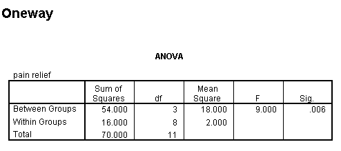
Here is what the output will look like.
Notice that the output is given in the standard ANOVA table output. SPSS doesn't tell you to reject or fail to reject the H0, nor does it give you the Fcrit. To make your decision about the H0 you must compare the p-value with your a-level. If the p-value is equal to or smaller than the your a-level, then you should reject the H0, otherwise you should fail to reject H0.

The ANOVA Table

Sources between groups within groups

Sum of squares SSb=S[(group mean - overall mean)2*n] SSw=S(group variance * n)

Degrees of Freedom dfb # of groups minus 1 dfw Total N - # of groups

Mean square The estimate of variability sum of squares divided by degrees of freedom

F statistis MS between / MS within

Significance level of F

Follow-Up Analyses

Recall that the ANOVA only tells us if there is any difference between the groups. If we want to know where the differences are, then we need to do some additional analyses. There are generally two kinds of additional analyses, planned means contrasts and post hoc tests. The "Planned" kind of additional tests are done if, in advance of doing your ANOVA, you know specifically what groups you expect to be different are (note: you should limit yourself to a fairly small set of comparisons). The "post hoc" tests are those that you do after you've done an ANOVA and found a difference and now want to konw what groups differ from one another.

Post Hoc Multiple Comparisons: Post hoc means "after the fact." "Multiple comparisons" means that all possible pairs of factors are compared. There are many options regarding post hoc tests on SPSS. However, some are more commonly used than others.

• LSD: the "least significant difference." This is the most liberal of the tests, since you are most likely to show significant differences in comparisons. This procedure is simply a series of t tests.
  • Scheffe and Bonferroni: most conservative of the tests.
  • Tukey: (HSD-Honestly Significant Difference). This calculates a number that represents the minimum difference between mean values in order to identify a significant difference. SPSS also has additional statistical information for this post hoc test.
  • Bonferroni procedure is a series of t-tests with an adjusted significance level
• After entering variables you wish to test, *Options
• *Descriptives, *Homogeneity of variances, *Continue
• * Post hoc test(s) you desire, *Continue, * OK

---

Using SPSS to do single factor ANOVA: Planned comparisons and Post hoc tests

Go to the Analyze menu and select the submenu Compare Means. In this submenu you'll see several tests. The one that we're interested in today is One-way ANOVA.

After selecting One-way ANOVA you'll get a window that looks like this. Here you should select the variables that you are testing. Your test variable is your dependent variable. Your group variable is the independent variable that assigns each subject to a group.

Click on the "contrasts" button to do planned comparisons. Click on the "post hoc" button to do post hocs.

• To do planned means comparisons you need to set up orthogonal comparisions. Notice that the SPSS box makes you enter some "coefficients". This is where the "orthogonal" part will come in. Basically it means that the coefficients that you enter have to sum up to zero. The coeffiecients are how you tell SPSS which groups to compare. You assign positive numbers for one (or more, but we won't worry about these more advanced comparisions) group and negative numbers to the group you want to compare it to. Then you assign zeros to the groups that you want to ignore. Consider the following set of coefficents.

  Coefficents Comparison 1, -1, 0 group 1 vs. group 2 1, 0, -1 group 1 vs. group 3 0, 1, -1 group 2 vs. group 3 To the right is what the output from SPSS looks like. The results of Comparision 1 (group 1 vs 2) is significant (p = 0.001) Comparison 2 (group 1 vs 3) is not significant (p > 0.05) Comparison 3 (group 2 vs 3) is significant (p = 0.001)

• To do post hoc tests is even easier. All you need to do is to click on the box of the kind of post hoc test that you want to do. Some of the most common are Tukey's HSD, Fisher's LSD, and Scheffe (a very conservative post hoc test). Notice that to do these tests you need to specify what level of a you want to use.

  The output for these three tests is presented below. For each, you will see the results of each pairwise comparision. For example, the Tukey HSD test, book alone vs. notes alone, is significant (p = 0.004), while book alone vs. borrowed notes is not significant (p > 0.05). The next set is notes alone vs book alone and notes alone vs borrowed, and the set after that is borrowed against book alone and borrowed against notes alone. The results for the other post hoc tests are aranged in the same way.

  

  Based on these results (either the planned comparisons, if we had some reason in advance to test the groups against one another, or the post hocs, if we found rejected the H₀ based on our ANOVA first) we can reject several of the alternative hypotheses:

  m1 not equal to m2 not equal to m3	REJECT
  m1 not equal to m2 = m3	REJECT
  m1 = m2 not equal to m3	REJECT
  m1 = m3 not equal to m2	FAIL TO REJECT