Outline

• Consider the logic & assumptions of hypothesis testing
• Discuss H₀ & H_A
• Create a distribution of sample means
• Determine likelihood of obtaining particular samples from populations

Hypothesis Testing

In the section of the course we learned to use the descriptive statistical procedures to describe distributions (and relationships between distributions). In the remainder of the course we will focus on inferential statistical procedures, which are used to make claims about the populations based on data collected from samples.

Hypothesis testing is an inferential procedure that uses sample data to evaluate the credibility of a hypothesis about a population.
Step 1: State the hypotheses and select a criteria for the decision Step 2: Collect a sample Step 3: Compute a test statistic Step 4: Compare the test statistic to a distribution to make an inference about the parameter and hence draw a conclusion about the sample

Let's look at each of these steps in more detail.

Step1: Make a hypothesis and select a criteria for the decision

- the assumptions are related to the stat test you'll do and we'll talk more about those as we discuss each individual test
- your hypothesis is an educated guess/prediction about the effect of particular events/treatments/factors (which result in differences between populations)
- your hypothesis may be general (e.g., this course will change comprehension abilities), or specific (e.g., this course will improve comprehension abilities by at least 10%).
The standard logic that underlies hypothesis testing is that there are always (at least) two hypotheses: the null hypothesis and the alternative hypothesis
The null hypothesis (H₀) predicts that the independent variable (treatment) has no effect on the dependent variable for the population.

The alternative hypothesis (H_a) predicts that the independent variable will have an effect on the dependent variable for the population

The hypothesis testing procedure assumes we are trying to reject the null hypothesis, not trying to prove the alternative hypothesis.

Why?
Generally, it is easier to show that something isn't true, than to prove that it is. This is especially true when we are dealing with samples. Remember that we aren't testing every individual in the population, only a subset.

Think about it this way. Suppose we had a hypothesis that all dogs have 4 legs. To reject this hypothesis, we'd need to have a sample which includes 1 or more dogs with more or fewer than 4 legs. To accept it, we'd need to examine every dog in the population and count their legs. It's much easier to get a sample to show it's wrong than to test the whole population to show that it's correct.

Example: Suppose that we know that in the US on average 30% of registered voters vote in each election. You want to try to increase that number with an ad campaign to try to get more people to vote. So we conduct the ad campaign before a major election and then record the percentage of voters that vote in that election.
What will our hypotheses be in this case? H₀ states that the independent variable will have no effect so our H₀ is that m = 30% (indicating no effect of ad campaign). Our H₁ is the opposite: that m will not equal 30%.

Alternatively, we could make a specific alternative hypothesis if we chose. This would change our H₀ too. Let's consider the specific case above where we expect that the ad campaign will INCREASE voters. This means that we expect higher voting rates for our sample than is in the population (30%). Here our H_a is that m > 30%. That means that our H₀ is m < or = 30%.

(1a) The diameter of a spindle in a small motor is supposed to be 5mm. If the spindle is either too small or too large, the motor will not work properly. The manufacturer measures the diameter in a sample of motors to determine whether the mean diameter has moved away from the target.

(1b) Census Bureau data show that the mean household income in the area served by a shopping mall is $52,500 per year. A market research firm questions shoppers at the mall. The researchers suspect the mean household income of mall shoppers is higher than that of the general population.

(1c) The examinations in a large psychology class are scaled after grading so that the mean score is 50. The professor thinks that one teaching assistant is a poor teacher and suspects that his students have a lower mean than the class as a whole. The TA's students this semester can be considered a sample from the population of all students in the course, so the professor compares their mean score with 50.

So part of the first step is to set up your null hypothesis and your alternative hypothesis (which we did above).

The other part of this step is to decide what criteria you are going to use to either reject or fail to reject (not accept) the null hypothesis. This is sometimes referred to as setting your a level (that's alpha level).

So consider the problem that we have. We have a sample and its descriptive statistics are different from the population's parameters. How do we decide whether the difference that we see is due to a "real" difference (which reflects a difference between two populations) or is due to sampling error?

To deal with this problem the researcher must set a criteria in advance.

What are the possible real world situations?
- H₀ is correct
- H₀ is wrong
What are the possible conclusions?
- H₀ is correct
- H₀ is wrong
So this sets up four possibilities (2 * 2):
- 2 ways of making mistakes
- 2 chances to be correct

	Actual situation
Experimenter's Conclusions	H0 is correct H0 is wrong Reject H0 Fail to reject H0 Type I error (oops!) correct (Yay!) correct (Yay!) Type II error (oops!)

The two kinds of errors each have their own name, because they really are reflecting different things.

Type I error (a, alpha) - the H₀ is actually correct, but the experimenter rejected it

- e.g., there really is only one population, even though the probability of getting a sample was really small, you just got one of those rare samples

Type II error (b, beta)- the H₀ is really wrong, but the experiment didn't give us the evidence we need to reject it

- e.g., your sample really does come from another population, but your sample mean is too close to the original population mean that you aren't can't rule out the possibility that there is only one population

In scientific research, we typically take a conservative approach, and set our critera such that we try to minimize the chance of making a Type I error (concluding that there is an effect of something when there really isn't). In other words, scientists focus on setting an acceptable alpha level (a), or level of significance.

The alpha level (a), or level of significance, is a probabiity value that defines the very unlikely sample outcomes when the null hypothesis is true. Whenever an experiment produces very unlikely data (as defined by alpha), we will reject the null hypothesis. Thus, the alpha level also defines the probability of a Type I error - that is, the probability of rejecting H₀ when it is actually true.

Note: In psychology a is usually set at 0.05

(2) A researcher would like to test the effectiveness of a newly developed growth hormone. The researcher knows that under normal circumstances laboratory rats reach an average weight of 1000 grams at 10 weeks of age. When the sample of 10 rats is weighed at 10 weeks, they weigh 1010 grams.

(a) Assuming that the growth hormone has no effect, what would a type I error be in this situation?
(b) Assuming that the growth hormone does have an effect, what would a type II error be in this situation?

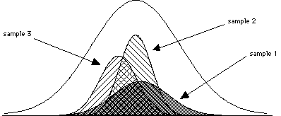
Step 2: Collecting your sample

When we discussed z-scores, we were using z-scores to locate a score or set of scores in the population.

Now we are dealing with situations in which we are looking not at single scores, but rather at samples of scores. These samples consist of scores that were randomly selected from a population of scores. As we saw in our earlier discussions of probability, random events are predicable in the long run. The following discussion and exercises demonstrate how we use this knowledge within the hypothesis testing framework to make claims about populations from samples.

Suppose that you take 3 different random samples from the same population. They are probably going to be different from one another. See the figures below for an example of what I mean.

The samples may have different shapes, different means, and different variability. So how do you figure out what the best estimate of the population mean is?

There are essentially an infinite number of samples that can be taken from a population if we sample with replacement (put the ones we choose back into the population each time). But the huge set of possible samples forms a simple, orderly, and predictable pattern (a sampling distribution). Because of this, we are able to base our predictions about sample characteristics on the distribution of sample means.

The distribution of sample means is the collection of sample means for all the possible random samples of a particular size (n) that can be obtained from a population.

In other words, what we want to do is look at all of the possible samples (of a particular size, this part is important) and make predictions based on the properties of all of them. We do this the same way that we've done in the past, we essentially find the average of those properties.

---

The Distribution of Sample Means

We can create a distribution of sample means by looking at all possible samples of a certain size (n) and considering the means of each of those samples.

Let's look at a concrete example:

Consider the following small population of scores: 2, 4, 6, 8

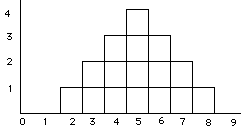
Because this population is so small we actually can know the mean (and variability): mean = (2+4+6+8)/4 = 5, but suppose that we didn't, and wanted to be able to make an estimate of this population from samples chosen from the population (like we do when we conduct a research study).

step 1: pick a sample size: for this example we'll pick samples of n = 2

- we'll talk more about sample size a little later, but typically the bigger your sample size, the more likely that your samples will be similar to one another (and to the population as a whole)

step 2: Because we selected such a small population, we can actually consider all of the possible samples that you could get (ignoring duplications resulting from sampling with replacement), and look at their distribution.

Okay, imagine that each score is a number on a tile. Put all four tiles in a bag. To create the first sample, pull out one tile, record the number on the tile, replace the tile in the bag, and then select the second tile (recall our sample size is 2) and record the value on that tile. The table below presents all 16 possible n = 2 samples that could result from this process along with the mean of each sample.

____________________________________
	scores		sample mean
sample	first	second	      ()  
1	2	2		2
2	2	4		3
3	2	6		4
4	2	8		5
5	4	2		3
6	4	4		4
7	4	6		5
8	4	8		6
9	6	2		4
10	6	4		5
11	6	6		6
12	6	8		7
13	8	2		5
14	8	4		6
15	8	6		7
16	8	8		8   

Distribution of the sample means
Now let's plot all of the different sample means (and provide a frequency distribution table). This is the distribution of sample means (where scores are means from the samples you chose).

f 2 1 3 2 4 3 5 4 6 3 7 2 8 1

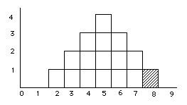
step 3: Now you're ready to answer questions like: What is the probability of getting a sample with a mean greater than 7? p( > 7) = ?



look at our distribution of sample means, we find that 1 out of 16 have a mean greater than 7. So that's our answer: 1/16 = .0625 = 6.25%

Properties of the distribution of sample means

• Mean:
  the average of all of the sample means will equal the mean of the population.

• Variability:
  the standard deviation of the distribution of sample means is called the standard error of the mean.

• Shape:
  the shape of the distribution of sample means tends to be a normal distribution. In fact, when n is large (around 30 or more), the distribution of sample means is almost perfectly normal.

The expected value of the mean

Open Dist. of Sample Means and click Begin.

The top distribution is the population distribution. We'll start a normally distributed population, which is set as the default. On the left are the descriptive statistics that describe this distribution.



From this population distribution we can draw random samples.

(3) Click on the "animated sample" button. This will randomly sample 5 individuals (n = 5) from the population (they'll drop down on to the graph immediately below the population graph). The applet will also compute the mean of this sample and plot the sample mean on the third plot (below the plot of the 5 individuals). In your worksheet, record the mean of the first sample. How does this mean compare to the mean of the population? How much sampling error is there (sampling error is the difference between the population mean and the sample mean)?

Click the "clear lower 3" button.

(4) Now let's try more samples. Click on the "5 samples" button. This will randomly select 5 samples (each sample will have n=5). The distribution of sample means plot (the third one down) will now have 5 sample means in it. What are 5 means? What is the mean of the distibution of sample means (the mean of the 5 sample means)? How does this mean of the distribution of sample means compare to the actual population mean?

Click the "clear lower 3 button.

(5) Now click the "10,000 samples" button. This will take 10,000 samples (of size n=5) and plot all of the sample means on the distribution of sample means plot. What is the mean of the distibution of sample means? How does this mean of the distribution of sample means compare to the actual population mean?

(6) State a generalization about the relationship between the population mean and the mean of the distribution of sample means.

---

Standard Error

The standard deviation of the distribution of sample means is called the standard error. The standard error is influenced by two factors: the variability of the population (s) and the sample size (n).

We'll consider each of these factors below:

(A) the variability of the population - the bigger the variability of the population, the more variability you'll have in the sample means.

large s big differences from the pop mean

small s small differerences from the pop mean

(B) the size of the sample - the larger your sample size (n), the more accurately the sample represents the population. This is known as the Law of large numbers.

think of it this way:

	- If I randomly selected 1 score, how accurately will that score predict the population's mean?
	- Suppose that I take 5 scores. Are things more accurate?
	- What about 100 scores?

These two characteristics are combined in the formula for the standard error.

standard error =

Now go back to the distribution of sample means applet again (or click below to open it again).

Dist. of Sample Means

We can use the applet to take samples of different sizes from the sample population for comparison. Set the bottom graph to take samples of size 20 (n=20) and to plot the "mean" (change the "none" to mean).

(7) Click on 1,000 sample button. This will take 1,000 samples of size n = 5 and 1,000 samples of size n = 20. What are the means of each of these sampling distributions? How do they compare? What are the standard errors (standard deviations of the sampling distributions) for each other?

The shape of the distribution of sample means.

Open up the distribution of sample means applet again.

Dist. of Sample Means

We can change the shape of the population distribution.

(8) Change the "normal" option to "skewed." As in the exercise above, sample two different sizes n = 5 & n = 20. Click the "1,000 samples" button. How do the shape of these distributions look? Are they skewed or fairly symmetrical? Which appears to be closer to Normal (hint: you can click the "fit normal" boxes to overlay a normal distribution)?

---

Central limit theorem All of these properties (shape, mean, variability) are covered in the Central Limit Theorem Central Limit Theorem: For any population with mean m and standard deviation s, the distribution of sample means for sample size n will approach a normal distriution with a mean of m and a standard deviation of as n approaches infinity. Note: for practical purposes this holds true for n > 30 (that is, for samples larger than n = 30).

---

Using the Distribution of Sample Means to Determine Sample Likelihood

Often we are not concerned with where a single individual is in a distribution, but rather where a sample is in the distribution of sample means. This tells us how likely we are to get that sample from a specific population. We can do this with the z-score distribution (and the unit normal table) if we know that the distribution of sample means is normal. (Remember that using the Central Limit Theorem, we know the distribution of sample means is normal if n is greater than 30 OR the population is normal.)

Example:

Consider the following situation. An instructor is interested in the IQ of her students. She has 9 students in her class and thinks that they are, on the average, really smart. What is the probability that the group of students has a mean greater than or equal to 112?

In other words, we don't want to know the probability of each individual having a score of 112 or better separately. Instead we want to know as a group, what is the probability of getting an average score of 112 or better.

We need to start by getting the population parameters

for the standardized IQ test: mean = 100, standard deviation = 15

Next we need to get the mean and standard deviation of the distribution of the samples (note: we'll assume a normal distribution because the original population distribution of IQ scores is normally distributed) so that we can calculate the z-score.

m = 100 (because the population mean is 100).

= = 15/sq. root of 9 = 15/3 = 5

Now we need to figure out the z-score that corresponds to this sample mean: the z-score formula pretty much looks like what we've used in the examples above (except now we're locating a sample in the distribution of sample means rather than finding a single score in a population): Z =


so for our example:

P( > 112) = P(Z > (112 - 100)/ 5 ) = P(Z > 2.4) = 0.0082

In other words, the probability that we'll get a sample of size n = 9 students with an average IQ equal to or greater than 112 is very small (0.0082). In our next labs we will extend this result to make claims concerning hypotheses about our population and our sample.

Does this answer make sense? Let's look at the pictures of our distributions.

Population distribution	- at first it looks wrong - it seems like 112 should be less than a z = 1, because 115 is where z should equal 1
Distribution of Sample means	- however, we must remember that this isn't the correct distribution to be looking at, we need to look at the distribution of sample means. -we know that the distribution of sample means has a standard error = 5 and a mean = 100. - So 112 should have a z >2

Let's look at a different kind of example.
Example:

How high a mean would a group of 25 have to have on IQ to be in the top 10% of the IQ distribution for groups of this size?
First we need to get the mean and standard deviation (i.e., standard error) for the distribution of the samples
population mean = 100

= = 15/sq. root of 25 = 15/5 = 3

Now we need to work backwards because we don't know the z-score. We can determine the z-score for the range based on the portion of the distribution we're looking for. We want the top 10% of the distribution. This corresponds to a proportion of .1000 for the distribution. If we look in the unit normal table, we find that .1000 corresponds to a z-score of 1.28 (that's as close to .1000 as we can get). You can verify this by looking at the unit normal table.

So for our example:

step 1: look at unit normal table for 10%

step 2: work backwards through the z-score formula to solve for

= z * + population mean = (1.28)(3) + 100 = 103.84

so, for a group of 25 people, they'd have to have a mean of just under 104 to be in the top 10%


(9) Suppose we think that listening to classical music will affect the amount of time it takes a person to fall asleep so we conduct a study to test this idea.

(a) Suppose that the average person in the population falls asleep in 15 minutes (without listening to classical music) with σ = 6 min, state the null and alternative hypotheses for this study.

(b) Assume that the amount of time it takes people in the population to fall asleep is normally distributed. In the study we have a sample of people listen to classical music and then we measure how long it takes them to fall asleep. Suppose the sample of 36 people fall asleep in 12 minutes. What is the probability of obtaining a sample mean of 12 minutes or smaller?

Next time: Finishing up hypothesis testing, steps 3 and 4