Outline

• Consider related samples
• Use Excel and SPSS to run related-sample t-tests

Hypothesis tests analyzed by related-samples t-tests

In the prior lab we examined how to use a t-test to compare a treatment sample against a population (for which s isn't known). In this lab we'll consider the case where the null population m isn't known and must also be represented by a sample (like the treatment m was in the one-sample cases. Today we'll consider situations where the two samples means come from related samples. The are two ways the samples can be related. In one case, there are two separate but related samples. In the other case, there is a single sample of individuals, each of which gets measured on the dependent variable twice.

Consider the following examples:

Example 1: Suppose that you want to compare married couples opinions about what makes a relationship work. So you decide to ask the husbands and wives to rate, on a scale from 1 to 10, how important communication is. You don't know the population means for these ratings. In this senario, even though you've got two groups (husbands and wives), the two groups are not independent. The members of each group are related to each other ("related" with respect to statistical selection issues, not religous or legal issues). So we need a t-test that takes the relatedness of the groups into condsideration.

Example 2: Suppose that you want to find out whether viagra impairs vision. Instead of comparing two separate groups, you decide to test the same set of individuals. In the first stage of the experiment you give your participants a placebo (a sugar pill that should have no effect on vision), and then test their vision. In the second stage, you give them viagra and then test their vision. So now you have the same people in both conditions. Clearly your samples are related, so again the t-test from the last chapter isn’t appropriate.

Example 3: Suppose that you are interested in the effect of studying on test performance. So you decide to use two groups of people for your study. However, you also decide that you want the two groups of people to be as similar as possible, so you match each individual in the two groups on as many important characteristics as you can. Again, the two samples are related, so the t-test from the last chapter isn’t appropriate.

In the first example, the situation has been decided for you, there is a pre-existing relationship between the two samples.

In the second and third examples, you, as the experimenter, make a decision to make the two samples related. Why would you ever want to do that? To control for individual differences that might add more noise (error) to your data. In Example 2, each individual acts as their own control. In Example 3, the control group is made up of people as similar to the people in the experimental group as you could get them. Both of these designs are used to try to reduce error resulting from individual differences.

A repeated-measures study is one in which a single sample of subjects is used to compare two (or more) different treatment conditions. Each individual is measured in one treatment, and then the same individual is measured again in the second treatment. Thus, a repeatted-measures study produces two (or more) sets of scores, but each set is obtained from the same sample of subjects. Sometimes this type of study is called a within-subjects design.

In a matched-subjects study, each individual in one sample is matched with a subject in the other sample. The matching is done so that the two individuals are equivalent (or nearly equivalent) with respect to a specific variable that the researcher would like to control. Sometimes this type of styd is called a related-samples design.

Okay, so now we know that for repeated-measures and matched-subject designs we need a new t-test. So, what is the t statistic for related samples?

Again, the logic of the hypothesis test is pretty much the same as it was for the one-sample cases we've already considered. Once again we'll go through the same steps. However, the nature of the hypothesis, and how the t is computed will change from our one-sample case.

All of the tests that we've looked at are examining differences. In the previous lab we were interested in comparing a known population with a treatment sample. Now we are beginning to consider cases when the null population m is unknown and must also be represented by a sample. The t-test for this lab also considers differences between scores from a related pair of subjects. Because the two scores for each pair are related, the differences are based on differences between each individual or matched pair.

Example of repeated-measures study (for review if you need it; otherwise, go to Excel section)

An instructor asks her statistics class, on the first day of classes, to rate how much they like statistics, on a scale of 1 to 10 (1 hate it, 10 love it). Then, at the end of the semester, the instructor asks the same students the same question. The instructor wants to know if taking the stats course had an impact on the students' feelings about statistics.

The results of the two ratings are presented below. D stands for the difference between the pre- and post-ratings for each individual (Post-Pre).
Note: = the mean of the differences

Student	Pre-test (first day)	Post-test (end of semester)	D
1	1	4	3	2	4
2	3	5	2	1	1
3	4	6	2	1	1
4	7	8	1	0	0
5	2	3	1	0	0
6	2	2	0	-1	1
7	4	6	2	1	1
8	3	4	1	0	0
9	6	6	0	-1	1
10	8	6	-2	-3	9
Σ	40	50	10	0	18
			Differences		SSD

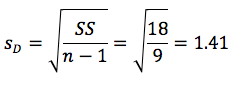
Mean difference for the sample = = 10/10 = 1.0

Process of hypothesis testing

Steps 1 & 2 : State H₀ & H_A and set a decision criterion.

Before we can state hypotheses, we need to know whether this will be a 1-tailed or 2-tailed test. All we are asking in this example is if taking statistics has an impact (any impact , in either direction) on the students' feelings about statistics. Since no direction of impact is predicted, this will be a 2-tailed test. Let's assume that α = 0.05.

H₀ will be a statement that taking statistics has no effect on a person's preference for statistics. If taking statistics has no effect, we would expect no difference between the pre-test scores and post-test scores, giving us a mean difference in the population of 0. So, we state:

H₀ --> μ_D = 0

The H_A will state the opposite case, that taking statistics does have an impact. Therefore, our alternative hypothesis is:

H_A --> μ_D ≠ 0

Step 3 : Sample statistics

Our sample is given above in the table with sample mean = 1.0 and we know μ _D = 0 (for the H₀), so we just need to figure out what is equal to. This is the estimated standard error of the difference distribution. So first we need to figure out the variance. We laready know that SS_D = 18.

standard deviation of the differences =

Now we can figure out the estimated standard error

 

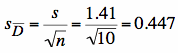
Step 4 : Test statistic

Now we need to calculate our t_observed.

As was the case in last lab, the overall form of the t statistic equation is the same, but the details are a little different.

df = 10 -1 = 9.

Step 5 : Compare t_observed with t_critical

Finding t_crit is the same as usual, look at the table. α = 0.05, two-tailed, df = 9 t_critical = ± 2.262


t distributions table


Our t_obs does not fit in the critical region: t_observed < t_critical (less extreme).

Fail to reject (i.e., retain) the H₀. No effect of taking the stats class on liking of statistics

Note: if we had made a directional hypothesis, that the stats class would increase preference of stats, we would have made a different decision about H0. Why would this happen? It would happen because we'd increase the power of our test to detect a difference (because we are looking at 0.05 in only one tail, instead of 0.025 in two tails). Our tcrit = 1.833. Our tobs would still be the same (2.24), so now in step 4 we would end up rejecting the H0.

Okay, what about Hypothesis testing with a matched-subject design?

Using SPSS to compute a related-samples (paired-samples) t-test

In SPSS, you proceed a little differently than you would with a one-sample t-test. We will use an example of 38 aggressive children who participated in an anger management and social skills training program. Each child’s aggression was assessed before and after treatment. You wish to know if the treatment was effective in lowering aggression. For the sake of simplicity, let’s make this a 2-tailed test because SPSS does not have a friendly way of doing one-tailed paired-samples t-tests. Thus, the null hypothesis is that the mean aggression scores are the same before and after treatment.

Go to Analyze and select Compare Means. In the submenu, select Paired-Samples T Test.
In the window for selecting variables, click on agression1 and the arrow for Variable1 and aggression2 (this is where the screen is shown) and the arrow for Variable2. Note that in SPSS, D = Var1 - Var2, so we needed to be careful about the order in which we enter the variables if we have a one-tailed hypothesis. Click OK.
Here is what the output will look like.
SPSS provides all of the following: mean, standard deviation, and standard error of each sample; M (sample mean1 - sample mean2), SD, and SE of the Differences; tobs, degrees of freedom, and p-value (Sig. 2-tailed). As we noted before, SPSS only provides 2-tailed p-values. Since we need a 1-tailed value to test our hypothesis, we get it by dividing the 2-tailed value in half. As we noted last time, SPSS doesn't tell you to reject or fail to reject the H0, nor does it give you the tcrit. To make your decision about the H0, you must compare the p-value with your α-level. If the p-value is equal to or smaller than the your α-level, then you should reject the H0; otherwise you should fail to reject H0. Notice that in in this case, the 2-tailed p-value would not be significant. This again demonstrates that a 1-tailed test is more powerful. For (α = .05), an observed t = 2.26 is in the critical region 1-tailed but not 2-tailed. Check the t-distribution table for critical values of t. One last thing to note: When SPSS gives you a p = .000, this does not mean that p actually equals 0. SPSS is rounding to three significant digits so if your output says p = .000, this really means that p is less than .001 (p < .001).

Now use SPSS to evaluate the following study.

A psychology instructor teaches statistics. She wants to know if her lectures are helping her students understand the material. So she tells students to read the chapter in the textbook before coming to class. At the beginning of class, she gives her students (n = 10) a short quiz on the material. Then she lectured on the same topic and followed her lecture with another quiz on the same material. Was there an effect of her lecture? Assume α = 0.05 level. The data are as follows:

Person	Pretest	 Posttest
  A	  15		15
  B	  11		13
  C	  10		18
  D	  11		12
  E	  14		16
  F	  10		10
  G	  11		19
  H	  10		20
  I	  12		13
  J	  15		18

Remember that SPSS automatically finds the difference of Var1-Var2. To have improvement be a positive score, enter Posttest as Variable1, so that the difference = Posttest - Pretest. .

				
Person	X1 (before)	X2 (after)
  A	  15		15
  B	  11		13
  C	  10		18
  D	  11		12
  E	  14		16
  F	  10		10
  G	  11		19
  H	  10		20
  I	  12		13
  J	  15		18