Outline
|
 |
Lab 18
|
|
Let's start with a brief review. In the last several labs we looked at ways to test samples.
We used one-sample t-tests to examine the same situation, except we don't know the population s, so we need to use an estimate (the sample standard deviation). The last lab used a different computational formula to calculate the observed t for two more situations: The logic of today's lab should seem similar to the last few. The overall logic is the same, we still use the t-distribution to find our critical values. However, things get a little more complicated, because of the situation that we are interested in. Now we are going to look at a situation where we are interested in the potential difference between two different populations, where each population is represented by a separate (and unrelated) sample. And again, we'll deal with situations in which we don't know the μ or s for either of these populations, so we'll have to use samples to estimate them.
So we'll use the same logic and steps for hypothesis testing that we used in the previous labs, and fill in the details of the differences as we go. Step 1: State your H0 and H1 and choose your criterion: α Step 2: Collect the
sample Step 3: Compute the
tobs for your sample Step 4: Compare tobs
to tcrit (or p to α) and make a decision
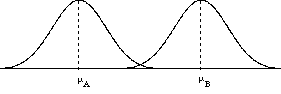
Let's start with Step 1: Figuring out your critera is exactly the same process as before, you pick what your field has decided as being an accepted level of alpha (chance of making a type I error). For our example, let's assume a = 0.05 The hypotheses are going to be a bit different, because the situation is different. Remember, that now we are making hypotheses about two different populations, not just comparing a treatment to what is known. For example, suppose that you want to compare two different treatments (e.g., two ways of studing, two different drugs, etc), or you want to compare two groups of people (e.g., men vs. women, young vs. old, etc.). So now, the hypotheses are about population A (men) and population B (women), and how they are different from one another. Suppose that we are interested in how tall men and women are.
Is this going to be a one-tailed test or a two-tailed test? In this case, we'll conduct a two-tailed test. We won't make a directional prediction. So the H0 hypothesis would be that men and women are the same height. That is, H0: μMen = μWomen - or - H0: μMen - μWomen = 0 Our alternative hypthesis would be that men and women are different mean heights. That is, H1: μMen not equal to mWomen - or - H1: μMen - μWomen not equal to 0
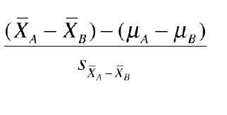
Step 2 : Criterion for decision: α= .05 Step 3 & 4: Sample & test statistics
Step 5 : Compare observed to critical value and make a decision about the null hypothesis
So now we compare the two t statistics. tobs = 5.22 Our observed (computed) t
statistic is much greater than the
critical t statistic; in fact, it is
greater than the largest critical t
reported in the t-table for df = 16, p =
.01, 2-tailed. Click on the table above to
find that value. So we feel confident in
rejecting the H0. There does
seem to be a difference between the
heights of men and women.
(1) A psychologist is interested in studying the effects of fatigue on mental alertness. She decides to study this question using an independent samples design. She randomly assigns individuals to two groups. Group 1 stays awake for 24
hours Group 2 gets to go to sleep After this period, each subject is tested to see how well they detect a light on screen (the dependent variable is the subjects' number of mistakes which reflects their mental alertness. So the higher the number, the less alert they are.). Here are the results from the two groups: n1 = 5 n2 = 10
Using an independent samples t-test, answer the question of whether fatigue adversely affects mental alertness (α = 0.05).
Using SPSS to compute independent-samples t-testsThe data entry for this test is different from that for related samples. There we had two measures taken on the same or related persons. Here we have only one dependent measure ("readingbefore" in the screenshots below) taken on two independent groups (two clubs "Latin" and "Sports"). There we had two columns for measures; here we have only one. But as a second column we need to identify which group the person belonged to. So we code group membership just as we could code club by indicating 1 = latin and 2 = sports.
(2): A psychology instructor at a large university teaches statistics. Because there are 22 students in the class, he has broken them into 2 groups. Each group has a different graduate assistant who is responsible for running separate breakout lecture and lab sections of the course. One GA has lots of experience teaching, while the other has more limited experience. The instructor wants to check for comparable learning across the two GAs, hoping to find no difference. The data below are the scores (out of 100) of the students on the first midterm. Assume an a = 0.05 level. The data are as follows (notice that one group has more students than the other):
Enter the data into SPSS. Test your H0 using an independent-samples t-test. Create a bar graph to show the results.
Lab Exercises 3 - 5 show how different designs affect the following set of data. Both tests will be to find any difference between treatments with α = .05. (These data can represent either 10 different participants or 5 participants tested in each condition.) Treatment 1 Treatment 2
(3) Assume that the data are from an independent samples experiment using two separate samples, each with 5 subjects. Use SPSS to test whether the data indicate a significant difference between the two treatments (assume a = .05). List each step of the hypothesis testing procedure. (4) Now assume that the data are from a repeated-measures design using one sample of 5 subjects, each of whom have been tested twice. Use SPSS to test whether the data indicate a significant difference between the two treatments (again assume a = .05). Remember that you'll have to change the way the data are entered in the data window.
(5) You should find that the repeated measures design and the independent samples design reaches a different conclusion. How do you explain the differences (hint: think about how sampling error is estimated for the two tests).
|
||||||||||||||||||||||||||||||||||||||||||||||||||||||||||||||||||||||||
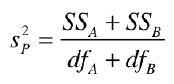
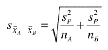
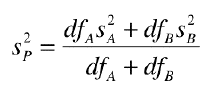 but we can
simplify this as:
but we can
simplify this as: