Outline

• cross tabulation of two
  categorical variables
• Chi-square test of independence

Cross tabulation and the Pearson Chi-Square Test

Both major and gender are categorical variables. And in this case, we're interested in whether there is a relationship between these two categorical variables: major and gender. The variables are measured in categories (thus, categorical variables). These two things put us at the bottom of our Which test? diagram: (1) we're looking for a relationship, and (2) we have categorical (nominal/ordinal, not interval/ratio) data. If we look at the bottom of the chart, these things will lead us to the Chi Square test.

One part of this test is a crosstabulation. Crosstabulation is a statistical technique used to display a breakdown of the data by these two variables (that is, it is a table that has displays the frequency of different majors broken down by gender).

The Pearson chi-square test essentially tells us whether the results of a crosstab are statistically significant. That is, are the two categorical variables independent (unrelated) of one another? So basically, the chi square test is a correlation test for categorical variables.

• A chi-square will be significant if the residuals (the differences between observed frequencies and expected frequencies) for one level of a variable differ as a function of another variable.
• The chi-square value does not tell us the nature of the differences
  

When do we use these methods?

• When we have categorical variables
  • Do the percentages match up with how we thought they would?
  • Are two (or more) categorical variables independent?

Hypothesis Testing with Chi-squared

• We test the null hypothesis that nothing interesting is happening (i.e., there is no relationship) versus alternative hypothesis that findings are interesting (i.e., there is a relationship).
  
• The null hypothesis can only be rejected if there is a .05 or lower probability that our findings are due to chance
  Hypothesis tests determine the extent to which our findings may be due to chance
  

  Example

  A manufacturer of watches takes a sample of 200 people. Each person is classified by age and watch type preference (digital vs. analog). The question: is there a relationship between age and watch preference?

  Setup our data in a "cross tabulation" of our two variables. The data are observed frequencies (f_o).

  		Watch preference
  		digital	analog	undecided
  Age	under 30	90	40	10
  	over 30	10	40	10

  Step 1: State the hypotheses and select an alpha level

  H₀: In the population, preference is independent of (NOT related to) age
  H_a: In the population, preference is related to age
  We'll set a = 0.05
  
  Step 2:
  • Compute your degrees of freedom
    df = (#Columns - 1) * (#Rows - 1)
  • Go to Chi-square statistic table and find the critical value
    For this example, with df = 2, and a = 0.05 the critical chi-squared value is 5.99
  Step 3: Collect your data and compute your test statistic
  Part 1: Obtain row and column totals, also called the marginals (in blue).

  		Watch preference
  		digital	analog	undecided
  Age	under 30	90	40	10	140
  	over 30	10	40	10	60
  		100	80	20

  Part 2: Compute the expected frequencies

  

  For people under 30

  • prefering digital watches: f_e = (100*140)/200 = 70
  • prefering analog watches: f_e = (80*140)/200 = 56
  • undecided watches: f_e = (20*140)/200 = 14

  For people over 30

  • prefering digital watches: f_e = (100*60)/200 = 30
  • prefering analog watches: f_e = (80*60)/200 = 24
  • undecided watches: f_e = (20*140)/60 = 6

  So let's enter the predicted (expected) values (in green) into our crosstabulation.

  		Watch preference
  		digital	analog	undecided
  Age	under 30	90 70	40 56	10 14	140
  	over 30	10 30	40 24	10 6	60
  		100	80	20

  Part 3: Compute the Chi-squared statistic

  

  • Find the residuals (f_o - f_e) for each cell
  • Square these differences
  • Divide the squared differences by fe
  • Sum the results

    

    So then add them up

    

    Here is the Table of Critical Values of the Chi Square Distribution.

  
  

  Step 4: Compare this computed statistic (38.09) against the critical value (5.99) and make a decision about your hypotheses
  
  • here we reject the H₀ and conclude that there is a relationship between age and watch preference

  ---

  1) Create a crosstabulation for the following data.

  Person number Sex Smoker 1 Male NonSmoker 2 Female Smoker 3 Male NonSmoker 4 Male Smoker 5 Female NonSmoker 6 Female NonSmoker 7 Male Smoker 8 Male NonSmoker 9 Male NonSmoker 10 Female Smoker 11 Female NonSmoker 12 Female NonSmoker 13 Female Smoker 14 Female Smoker 15 Female Smoker

  16 Female NonSmoker 17 Male NonSmoker 18 Male Smoker 19 Female NonSmoker 20 Male NonSmoker 21 Female NonSmoker 22 Male NonSmoker 23 Male NonSmoker 24 Male Smoker 25 Male Smoker 26 Female Smoker 27 Female NonSmoker 28 Male NonSmoker 29 Female NonSmoker 30 Female NonSmoker

  2) Compute the marginals and expected values for (1).

  3) Gender differences in dream content are well documented. Suppose that a researcher studies aggression content in the dreams of men and women. Each subject reports his or her most recent dream. Then each dream is judged by a panel of experts to have low, medium, or high aggression content. The observed frequencies are shown in the following table. Is there a relationship between gender and the aggression content of dreams? Test with a = 0.01. Be sure to state your hypotheses.

  		Aggression content
  		low	medium	high
  Gender	Female	18	4	2
  	male	4	17	15

Computing Crosstabs and Chi-square in SPSS

Excel has a formula for Chi-square (CHITEST), but it requires entering expected frequencies. It is inefficient to have to calculate these, so we cover only the Chi-square test in SPSS.

Choose Analyze, Descriptive Statistics, Crosstabs
Select your categorical variables Enter one in Row and the other in Column Click on the Statistics button, check the Chi-square option and click Continue to return to the Crosstabs page.

Click on the Cells button. Counts, Observed is checked by default. Check Counts, Expected. (This is not a necessary step, but it is useful to see the Expected Counts.). Click Continue to return to the Crosstabss page. Check Display clustered bar charts. Now click OK to run the analysis.
Note: if you would like the expected frequencies and residuals, you can specify those using the Cells button.
	Expected Frequencies Check Expected in the Counts box. One of the reasons that you want to see the expected frequencies is that the χ2 test is only accurate if the expected frequencies are sufficiently large (The observed frequences can be any value, though.). As a rule of thumb, we check to see if all of the expected frequencies are at least 5. Residuals Unstandardized residuals are the differences between the expected and observed frequencies. Standardized residuals are the unstandardized residuals after they have been converted to z-scores. This makes it easy to see which cells are extremely different from what the null hypothesis predicts.
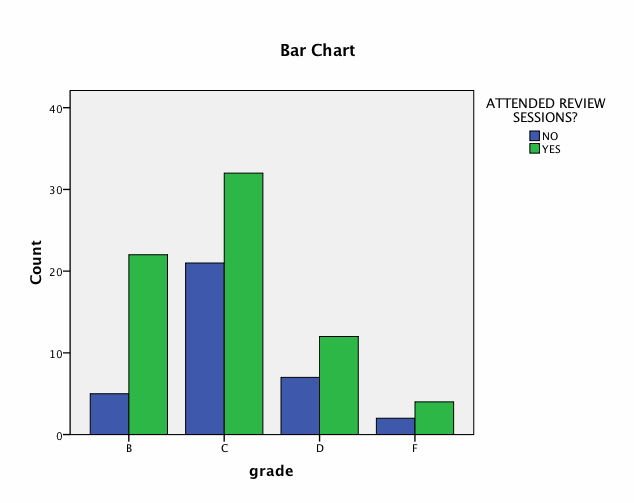
Output: Here is some sample output looking at a crosstab of Grade and review (attendance at the review session or not) from the gradebook.sav file. The Crosstabulation table shows frequencies of one variable for each level of the othe. Count refers to the observed frequencies. Expected count refers to the expected frequencies in the cells given the marginal totals.
Output shows the (Pearson) chi-square value and its significance level ("Asymp. Sig."). It provides a note about cells with low frequencies, since theintroduce more error into the test. You have the option of combining cells to eliminate such low frequencies. Here the chi square is not significant (p is greater than α = 0.05), so we would fail to reject the H0 that final grade and review session attendance are independent. (In other words, there is not a relationship between the two variables.)
Clustered bar charts or tables are the most common way to present data from crosstabulations. SPSS plots these charts as part of this program. they are the same as you could make yourself under Graphs.

For the following two questions download the file students.sav.

4) Were juniors and seniors more likely than freshmen and sophomores to attend the review sessions? Provide a bar chart showing the breakdown. Assuming an a = 0.05, test whether these variables are independent. Remember to state your hypotheses.

5) Were men more likely than women to do an extra credit assignment? Report the number of people who did and didn't do the extra credit project broken down by gender. Assuming an a = 0.05, test whether gender and extra credit participation are independent. Remember to state your hypotheses.

Assumptions of the Chi-Square

Categories are independent (no overlap)
Must have an expected count of at least 5 in each cell
Remember that large samples mean large chi-squares, thus making it easier to find a significant chi-square (this is called power)