• The relationship between correlation and regression
• The equation of a line
• Scatterplots

Basics

Correlation and regression procedures share a number of similarities.
Correlation describes the relationship between two continuous variables
Regression allows one to predict scores on one variable given a score on another

Both correlation and regression test the null hypothesis that the two variables are independent of one another

1) The direction of the relationship
2) The form of the relationship
3) The degree of the relationship


Regression will give us these properties as well as allows us to make specific predictions about one variable, based on what we know about another variable.

Prediction - if we know that two variables are strongly related, then we may be able to predict the value of one, based on the value of the other.

e.g., if you know that ultrasound measurements of a baby's head are positively correlated with birth weight, then you can make an educated guess of the baby's birth weight by measuring the baby's head from an ultrasound

The equation for a line

Let's start by reviewing some old geometry. Consider the follwing graph.

at X = 0, Y = 1 at X = 1, Y = 1.5 at X = 2, Y = 2.0 at X = 3, Y = 2.5 at X = 4, Y = 3.0 So as X goes up by 1, Y goes up by 0.5. This is called the slope (b). This is a constant. The intercept (a) is the value of Y when X = 0. This is also a constant. We can describe the line in the following linear equation: Y = bX + a ---> Y = (.5)X + 1.0 in other words, using the linear equation, we can determine the value of Y, if we know the values of X, b, & a - recall that predicting Y based on X is one of the main things that this chapter is all about

Scatterplots

Okay, now let's return to our scatterplots. Let's start with the case of a perfect positive correlation (r = 1.0).

When we do a regression analysis, what we are doing is trying to find the line (and linear equation) that best fits the data points. For this example it is pretty easy. There is only one possible line that makes sense to fit to this set of data.

Now let's look at a case when the correlation is not perfect.

Now it isn't as easy. Clearly no single straight line will fit each data point (that is, you can't draw a single line through all of the data points). In fact it is not too hard to imagine several different possible lines fitting to this data. What we want is the line (and linear equation) the fits the best.

Getting SPSS to make a scatter plot and put a least squares regression line on our scatterplot

Making the scatterplot
• The first step in creating a scatterplot for regression is to remember that the variable that you are predicting goes on the Y-axis. The predictor goes on the X-axis (if you're looking at correlations rather than regressions it really doesn't matter which goes where). For example, if you want to predict weight with height, then you should put weight on the Y-axis and height on the X-axis.
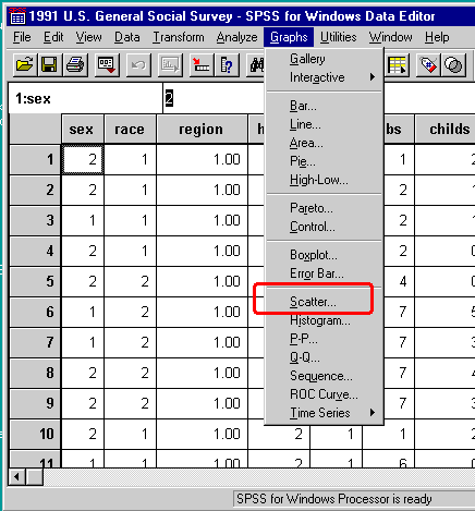
• To have SPSS create the scatterplot click on the scatterplot submenu under the graphs menu. You will find scatterplot under the graphs menu.

  

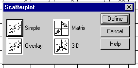
  	Select "simple" scatterplot
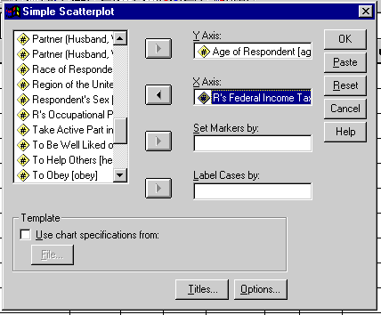
  	To assign your X and Y variables you need to select them from the variable listing and insert them into the X and Y axis. You can also mark the indivdual data points by adding a categorical variable into the "set markers by" field. .

  This will open up an output window and insert your scatterplot.

Fitting the line
• After the scatterplot is created, we can fit a least squares regression line on the plot by using the Chart Editor. Recall that to open the chart editor you need to double click on the graph of interest. This will open up a new window, the chart editor.
• Now you need to go into the "Chart" menu and select "options". Click here.
• This will open up the options window. In this window you should click on "Total" in the fit line box (upper right corner). Then click 'OK'. That's it, your scatterplot should now have a line on it.

Least Squares Regression

What does it mean to be the line that "best fits" the data?

Basically what we want to do is minimize the error. That is, the line that differs the least from all of the data points is the best fitting line.
Remember what the line is, it is a formula (a linear equation) that predicts the value of Y given X, a (the intercept), & b (the slope). So what we want to do is pick the line that gives the best estimate of Y. That is, the line that makes the smallest error in estimating all of the Y values.

So how do we do this?
We find the least-squares solution. There are two components to this computation, the slope of the line (b), and the intercept of the line (a).
• The formula for the slope of the best fitting line is:
  b = SP/SS_X

  Note: Your book gives a different formula for the slope. It is mathematically identical to the one above. To decide which to use, look at what information you know.

• The formula for the intercept of the best fitting line is:
  a = - b

  We've already computed all of these parts. So let's revisit the example that we used for correlations.


So SP = 14; SS_X = 64; SS_Y = 4

What is the regression equation for this data?

slope = b = SP/SS_X = 14/64 = .22

intercept = a = - b = 2.0 - (.22)(6.0) = .68

So the regression equation is:

= .22(X) + .68

Calculating the residuals (the error around the line)

So now we have our regression equation for the data from our example. We can use this equation to predict Y, given values of X. However, we need more information to complete our description of the relationship between the two variables.

• If the relationship between the two variables is perfect (r = +1.0) then all of the points are pefectly predictive, they all fall on the line, and so there is no error (no residual).
• If the predicted value is not perfect (r not equal to ± 1.0)then few (if any) points will actually fit exactly on the line. So there are differences between the observed values of Y and the predicted values of Y (as defined by the line). These differences are referred to as residuals, or error around the line.

Consider these two scatterplots. The equation for the line is identical for both, however the relationship between the variables (X&Y) are differrent. The relationship is weaker in the first plot relative to the second. That's because there is more error around the line in the first. This is why we must report not only the equation for the line but also a measure of error.

(). The standard error of the estimate describes the typical error in using to estimate Y.

To get this we'll look at each point, and compare the actual value for Y with the predicted value of Y (which is called (pronounced "Y-hat")

distance = SSerror = total squared error = We get the values from the line, and the Y values from the actual data points We need to do this for all of the values of a and b.

How do we compute the standard error of the estimate ?

First we need our total squared error

SS_error =

Then we'll divide that by our degrees of freedom (which gives us a measure of variance, or mean squared error)

SS_error / df

remember that df = n - 2

Then finally, to get the standard error of the estimate we take the square root of the whole thing (like standard deviation)

So in the end we end up with:

S_error = = =
So for our example:



= .22(X) + .68

S_error = = = = .559

Another way to compute S_error is to use the correlational information (if you've got it handy).

SS_error = (1 - r²)SS_Y = (1 - (+0.875)²)(4) = (1 - .766)(4) = .9375

S_error = = = .559

Residual Plots

The sum of the residuals should always equal 0 (as should the mean). This is because the least squares regression line splits the data in half, half of the error is above the line and half is below the line.

However, in addition to summing to zero, we also want there the residuals to be randomly distributed. That is, there should be no pattern to the residuals. If there is a pattern, it may suggest that there is more than a simple linear relationship between the two variables.

Residual plots are very useful tools to examine the relationship even further. These are basically scatterplots of the residuals () against the Explanatory (X) variable (note: plots of the residuals against other variables can also be enlightening). Consider the three examples below (note: the examples actually plot the residuals that have transformed into z-scores).

The scatterplot shows a nice linear relationship. The residual plot shows that the residuals fall randomly above and below the line. Critically there doesn't seem to be a discernable pattern to the residuals.

The scatterplot also shows a nice linear relationship. However, the residual plot shows that the residuals get larger as X increases. This suggests that the variability around the line is not constant across values of X.This is refered to as a violation of homogeniety of variance.

The scatterplot shows what may be a linear relationship. The residual plot, however, suggests that a non-linear relationship may be more appropriate (see how a curved pattern appears in the residual plot).

Getting residual plots in SPSS

Getting SPSS to make these kinds of residual plots is a two step process.

The first step is to save the residuals.

This is done when SPSS performs the regression analysis. At the bottom of the regression window there is a button labeled "save".
When you click the save button, this window opens. Click the save residuals box in the upper right corner.

This will save a new column in your datafile. It contains the residuals of your linear regression analysis.

The second step is to make a scatterplot, using the residuals as your Y-axis variable and the X variable as your X-axis.

The General Linear Model

The General Linear Model brings samples and population issues back into the picture. The least squares regression line that we've discussed up until this point can be considered the sample estimate of the true regression equation for the population.

The notation will change a little bit. Now we'll refer to the slope of the line as B₁ and the intercept as B₀. So the equation for the line is:

As was discussed above, we also need a measure of the error (variability) around the line. This will we signified by the Greek letter epsilon. So the full equation will be:

This equation describes a statistical model of the data. The portions of the equation sometimes described as consisting of the FIT and the RESIDUAL. The fit consists of the linear equation and the RESIDUAL is the error (the variability that isn't explained by the linear equation).

Using Regression to Test for a Relationship

The test of the regression model basically boils down to a test of whether the slope is equal to zero. The steps are similar to previous tests of hypotheses.

The null hypothesis, H₀: B₁ = 0.

That is, if the slope is zero, then there is no relationship between X and Y.

The degrees of freedom are: df = n - 2 (where n = the number of XY pairs)

There are several tests of the model. The most important two are the ANOVA and one of the coefficient t-tests. For Bivariate Regression, these two tests yield the same outcome (the F from the ANOVA is the square of the T from the T-test). For our current purposes, we'll just focus on the t-test of the slope.

Here is the breakdown of the components of the ANOVA table:

SPSS will also perform a t-test to test a hypothesis for the intercept (H₀: B₀ = 0), but these results are rarely used.

Using SPSS to preform Regression

If you'd like to follow along the example with the SPSS data file that it is based on, you may download the height.sav datafile.

We can also use our regression technique to test for a significant relationship between two variables. Remember that when we perform a regression, we calculate a slope (b) for the "best fit" line to describe the data. SPSS provides a test (a t-test) to determine if the slope (b) is significantly different from 0 (indicating that there is a linear relationship between the two variables).

To review:

• Under the "Analyze" menu select "regression". Click here.
• Under the "regression" submenu select "linear". Click here.
• Enter your dependent (response) variable and your independent (explanatory) variable into the appropriate fields. Click here.

  Note: you can add more than one explanatory variable at a time. This is called "multiple regression". This is a more advanced topic that we may talk about in detail later in the course. For now, just do regressions with one independent variable at a time.

  Look at the output below.

  Note: the regression analysis also gives us the power to do more than just get the equation for the line. Because of this, our output will have a lot of information in it. Be prepared to have to sift through it to get the information that we want.

  The output produced by the Regression command includes four different values:

  • A score which measures the strength of the relationship between the DV and the IV. This is designated with a capital R (the same as the bivariate correlation "r").
  • A probability value (p) associated with R which indicates the significance of that assoc.
  • R square, which is the proportion of variance in one variable accounted for by the other variable.
  • The information for the Least Squares Regression curve are highlighted in yellow here (but won't be in your SPSS output). They correspond to the "Unstandardized Beta weights" for the intercept (constant) and the slope (your variable name). The constant (intercept) and the coefficient (slope) for the regression equation (these are typically called the betas).
  The slope (B₁) is highlighted in yellow below. It is the value listed with the explantory variable and is equal to 1.193 in the output. In the same row on the right side of the output, you can see columns for t and Sig. values. This is a t-test (with the appropriate p value) to indicate if the slope is signficantly different from 0. In this case, it is, because p is rounded to .000 in the output (p < .001). This means that there is a significant linear relationship between the two variables tested here.

So for this relationship the linear equation (the FIT part of the model) is:

Some facts and cautions about correlation and regression

For practice you may download the bear.sav file to answer the following questions. The datafile includes data about bears. There are 6 variables: age, neck diameter, length (from head to toe), chest diameter, weight, and gender.

1) Relationships between variables

a) Which two variables are most strongly related to one another? Describe the nature of the relationship.

b) Describe the form of the relationship between age and length. Offer an explanation/interpretation of what this relationship suggests about the length of bears as they age.

c) Examine the neck by length scatterplot. There are three possible outliers. What sex are these bears? If those bears were excluded (removed) from the analysis, would the correlation get stronger or weaker?

d) Examine the relationship between age and weight. Is there more variability in weight for young or adult bears? Explain your conclusion.

e) Use regression to predict a bear's weight based on their chest diameter. Is the slope positive or negative? Give the regression equation for the "best fitting line." Suppose that you found a new bear with a chest diameter of 33 inches, what would you predict that bear's weight would be (using your regression equation)?

Below, I've provided a link to a very nice tool for getting a feel for regression (and residuals). On this page, you can place points on a scatterplot. The page will automatically compute the least squares regression line corresponding to the points (you can have a line put on too). Additionally, you can have it open up another window on which it will display a residual plot. I stongly suggest that you play with this.

Some suggestions for "play activities":

• Enter data for a strong positive relationship. Examine the residual plot. Add an outlier, what happens to the correlation and slope of the line? What happens to the residual plot?
• Enter data for a weak negative relationship. Examine the residual plot. Add an outlier, what happens to the correlation and slope of the line? What happens to the residual plot?

• Enter data for a curved relationship. Examine the residual plot.
It takes a little time to load the page, so be patient.