• Gravetter, F. J., Wallnau, L. B. (1996). Statistics for the Behavioral Sciences:
  A First Course for Students of Psychology and Education, 4th Edition. New York: West Publishing.
  

  ---

  Chapter 6: Probability Why probability? Because we're now moving towards talking about inferential statistics, that is making claims about populations based on information from samples.

  So we'll start this chapter by talking about probabilities. Then we'll move onto a discussion of normal distributions. And finally, we'll integrate the two topics.

  We deal with probabilities everyday.

  - lotto tickets, weather forcasts, medical reports on the news (e.g., risks of cancer)

  In a situation where several different outcomes are possible, we define the probability for any particular outcome as a fraction or proportion. If the possible outcomes are identified as A, B, C, D, and so on, then:

  	Probability of A = number of outcomes classified as A
  	   		   total number of possible outcomes
  

  - making it more concrete:

  you are playing card wars with your kid sister, each of you has your own deck of 52 cards. She picks the King of spades from her deck. What are the odds that you'll pick the King of Spades from your deck?

  	prob of K-spades =   ____picking the King of Spades ___
  			    total number of possible cards picked
  
  		         =  1 / 52
  

  Notation of probability: p(King-spades) = f / N

  Notice that we've already seen this f / N formula before. Does anybody remember it?

  Think back to our frequency distribution tables. We used this formula to figure out proportions. In fact probabilities are most often given as proportions (but can also give them as fractions or percentages). We'll come back to this in a little bit.

  However, for this definition of probability to be accurate, the selection of individuals (sampling) must be obtained by random sampling

  A random sample must satisfy two requirements:

  1. Each individual in the population has an equal chance of being selected.
  2. If more than one individual is to be selected for the sample, there must beconstant probability for each and every selection.

  so let's reconsider our card game situation

  - suppose that you are a card cheat and you stacked the deck so that all of the high cards are on the top, and the low cards are on the bottom.
  
  So you turn over the top card, and surprise, it is a high card.
  Was this a random sample?
  
  No, because not every card had an equal chance of being selected (becasue the low cards were not near the top of the deck).
  - suppose that you and your sister are playing with one deck of cards.
  Now she picks the King of Spades. Now you pick from the remaining cards.
  Is your chance of picking the King of Spades still 1 in 52?
  How about 1 in 51?
  No, because she already picked the King of Spades, so it isn't available for future selection. - what you need to do to have a random sample, is replace the King of Spades into the deck.

  Sampling with replacement - a sampling method in which each sample (individual) is replaced into the population before the selection of the next sample (individual)

  Okay, let's return to frequency distributions and how they relate to probability.

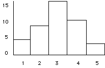
  Consider the following distribution.

  ___________________ X f_ p_ 5 2 .05 4 10 .25 3 16 .40 2 8 .20 1 4 .10

  You can see that our proportion column corresponds to probability. Which in turn correspond to the area under the curve for those intervals.

  Imagine that they are numbered tokens in a bag, and that your task is to reach in and pull one out.
  What is the probability of selecting (sampling) a 3?

  p (3) = f / N = 16 / 40 = .40

  What is the probability of selecting (sampling) a 5?

  p(5) = f / N = 2 / 40 = .05

  What about more complex questions?

  What is the probability of selecting a token with a value greater than 2?

  p(X > 2) = ? .05 + .25 + .40 = .70

  What is the probability of selecting a token with a value less than 5?

  p(X < 5) = ? .10 + .20 + .40 + .25 = .95

  What is the probability of selecting a token with a value greater than 1 & less than 4?

  p(4 > X > 1) = ? .20 + .40 = .60

  Now we'll move onto a different distribution, the Normal Distribution, and see how we work with probabilities. If a distribution is normally distributed then it is described in the following way: X ~ N ((, ().
  Normal distribution is a commonly found distribution that is symmetrical and unimodal. It is defined by the following equation:

  				Y = 
  
  

  

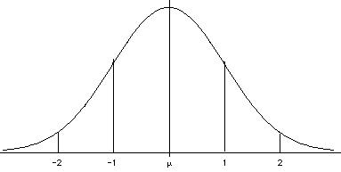
  A few things to note about Normal Distributions.

  • Not all unimodal, symmetrical curves are normal, but a lot are
  • For this class, we won't worry about how close a distribution is to normal, in fact for most of the course we'll assume that the distribution is normal
  • A smooth curve like that above is refered to as a density curve (rather than a frequency curve)
  • The area under (any density) curve must sum to 1. Why? remember that the area under the curve refers to the probabilities (or proportions) and the total probability must equal 1.
  • The normal distriution is often transformed into z-scores.
  • For a normal distribution:
    34.13% of the scores will fall between m and 1 stdev.
    13.59% of the scores will fall between 1stdev & 2stdev.
    2.28% of the scores will fall between the 2stdev & 3stdev.

  

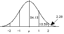
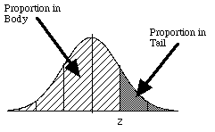
  An important tool that we'll use is the unit normal table. You'll find it in the appendix of your book (pg. A24-A26). In this table are a bunch of z-scores and proportions for the Standard Normal Distribution (which is the z-score standarized Normal distribution; N(0,1)). In other words this table allows you to figure out the area under the curve (and thus the probability of sampling) at nearly every position on the curve (defined in z-scores).

  Using the unit normal table.

  Column A - the Z-score in question
  Column B - the p(Z < z) - the proportion of the distribution in the Body
  Column C - the p(Z > z) - the proportion of the distribution in the Tail
  

  (A) z ____ 0.00 0.01 : : 0.30 0.31 : 1.00 :

  (B) Proportion in Body 0.5000 0.5040 : : 0.6179 0.6217 : 0.8413 :

  (C) Proportion in Tail 0.5000 0.4960 : : 0.3821 0.3783 : 0.1587 :

  Notice that z = 1.0 = .5000 + .3413 = the median + the 34.13% that we mentioned before So by using the table, we can an ask about different areas under the curve. And similar to last chapter, we can go in both directions. That is, from the table of z-scores to probabilities and/or from probabilities to z-scores.

  Note: Don't underestimate the value of drawing a picture of the distribution and trying to just "eyeball" the answer (in addition to doing the math). It just may save you from making a mistake.

  Here is the "best" way to find a probability from the table:
  step 1: sktech the distribution, showing the mean & standard deviation
  step 2: sketch the score in question, being sure to place it on the correct side of the mean & roughly the correct distance from the mean
  step 3: read the problem again to see if you need the probability of getting a score > or <. Shade this area on your sketch.
  step 4: translate the X score into a Z-score
  step 5: Use the correct column (and sign) to find the probability in the unit normal table.

  Examples:

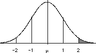
  What is the probability of having an IQ of 130 or above? p(X > 130)? for IQ scores m = 100, s =15 z = (130 - 100)/15 = 2.0 --look at the table--> need Column C p = 0.0228
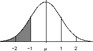
  What is the probability of having an IQ of 85 or less? p(X < 70)? for IQ scores m = 100, s =15, z = (70 - 100)/15 = -1.0 --look at the table--> need Column C p = 0.1587

  Here is the "best" way to find a Z-score from a probability:

  step 1: Sketch the normal distribution
  step 2: shade the region corresponding to the required probability
  step 3: locate the probability in the correct column of the table
  step 4: label the edge of the shaded region with the z-score from the step above
  step 5: compute the corresponding raw score (X).
  
  ** keep in mind that the percentile rank is equal to the probability of being at or below a given score. Thus, percentile ranks less than 50% refer to the lower tail.

  Example:

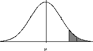
  What IQ score do you need to have to be in the top 5% of the population? The upper-tail is needed. p = 0.05 ---- look at the table ---> z = 1.65 so X = (1.65)(15) + 100 = 124.75

  Sometimes we need to find the probability that X will fall between two scores rather than simply above a score or below a score.

  step 1: Sketch the curve & shade the region of interest
  step 2: Translate both scores to Z-scores
  step 3: Look up the probabilities of scoring < or > each of the two z-scores
  step 4: Add (or subtract) the probabilities accordingly
  

  Example:

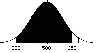
  What is the prob. of scoring between 300 and 650 on the SAT? recall: m = 500, s =100 p(z < (650 - 500) = p(z < 1.5) = 0.9332 100 p(z < (300 - 500) = p(z < -2.0) = 0.0228 100 the .9332 from 650 includes the lower tail, so we determine the proportion in the lower tail, and subtract that p(300 < z < 650) = .9332 - .0228 =.9104

  And finally, you might want to know what percentage lies outside two points (essentially the opposite of the last situation).

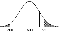
  What is the prob. of scoring lower than 300 or higher than 650 on the SAT? recall: m = 500, s =100 p(z > (650 - 500) = p(z > 1.5) = 0.0668 100 p(z < (300 - 500) = p(z < -2.0) = 0.0228 100 the two numbers both reflect the proportions in the tails, so we just need to add them together p(300 < z < 650) = .0668 + .0228 =.0896

  Another thing that you can use the unit normal table for is to find percentile ranks and interquartile ranges

  Examples:

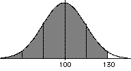
  What is your percentile rank if you have an IQ of 130? for IQ scores m = 100, s =15 z = (130 - 100)/15 = 2.0 --look at the table--> need Column B p = 0.9772 --> percntile rank 97.72
  What is the interquartile range for the SAT? recall: m = 500, s =100 --look at the table --> find 25% & 75% 0.25 = a Z-score of -0.67 0.50 = a Z-score of +0.67 X = Zs + m = (-.67)(100) + 500 = 433 = (+.67)(100) + 500 = 567 IQR = 567 - 433 = 134

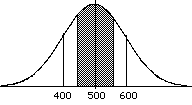Note there is a short-cut for figuring out the IQR. Since the range is always + .67s, then you can compute the IQR as being (2)(.67)(m)

example: for SAT: (2)(.67)(100) = 134

Let's talk about another very common distribution, the binomial distribution. This is a distribution that results when there are only two possible outcomes for a particular situation. For example, flip an unbiased coin: heads or tails, answer a yes/no question, a person either survives or dies, etc. The binomial distribution is denoted as: B(n,p), and it has a compex equation too (which you also don't need to learn).

As it turns out the normal distribution is a good approximation of the binomial distribution, if the n is big enough. We'll get back to this in a bit.

Let's think of the binomial distribution in probability terms.

two categories: A & B
p = p(A) = the probability of A
q = p(B) = the probability of B

So what does p + q = ?? ----> 1.0

n = the number of individuals (or observations) in the sample
X = the number of times a category A event occurs in the sample

Using this notation, the binomial distribution shows the probability associated with each value of X from X = 0 to X = n.

Example 1

consider the lottery. Suppose that you could win 1 million dollars. And that each ticket costs a dollar. With a 1 in a million chance of winning, then P(a) = 1/1,000,000 and P(b) = 999,999/1,000,000.

So the probability of winning is .000001
The probability of losing is .999999

now let's start figuring out how many tickets to buy.

n (# of tickets purchased) 1 10 100 1,000 10,000 100,000 1,000,000

P(winning at least once) 0.000001 0.00001 0.0001 0.0009950 0.00995017 0.09516263 0.63212074

Notice that even if you spend $1,000,000 to buy 1,000,000 tickets, your chances of winning are still only about 63%.

Let's consider another example: the flipping of a coin. A = heads; B = tails

p = p(A) = 1/2

q = p(B) = 1/2

suppose that n = 2 (that is, we flip the coin twice), how many possible outcomes are there B(2, 0.5)? four

toss 1 toss 2 # of heads heads heads 2 heads tails 1 tails heads 1 tails tails 0

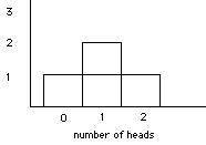so what is the probability of flipping two heads? 1/4 what is the probability of flipping no heads? 1/4 what is the probability of flipping only 1 head? 2/4 what is the probability of flipping at least 1 head? 3/4

Okay, now let's suppose the n = 6. Now how many possible outcomes are there? 64 the secret formula is: 2n

t1	t2	t3	t4	t5	t6		#heads
head	head	head	head	head	head		     6
head	head	head	head	head	tail		     5
head	head	head	head	tail	head		     5
head	head	head	head	tail	tail		     4
   :	   :	    :	   : 	  :	  :		     :
tail	tail	tail	tail	tail	tail		     0

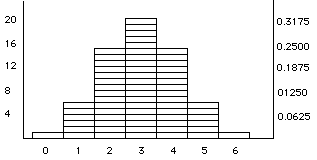
Recall, that I mentioned that the binomial distribution, when n is high, the normal distribution is a good approximation for the binomial distribution. Look how close it is with an n = 6 (pn = .5*6 = 3).

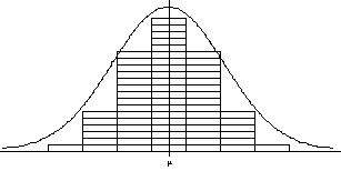
So when n = large (pn > 10) and (qn > 10), we can approximate the binomial distribution with the normal distribution.

Mean: m = pn

Standard deviation: s =

					z =      

We can use the z-scores from the unit normal table. However, it is important to remember that the value of X on a Normal distribution is really an interval, not a point, so we need to consider the real limits when approximating the binomial distribution. That is, we are using a continuous distribution (Normal) to estimate values in a discrete distribution (the binomial distribution).

example: Sometimes a student is admitted to college who cannot or will not make it through college. If the probability of dropping out for any one persone is 0.10, then what is the probability of having more than 15 students in a class of 100 drop out?

n = 100	p = 0.10	q = 0.90	np = .10*100 = 10  	nq = 90


mx = pn  = 10		sx =  = sqroot (100*.10*.90) = sqroot (9)  = 3


	p(X > lower real limit of 15)	= P(X >  14.5) 


					= P(Z >  14.5-10) 
						  3.0


					= P(z >  1.5) 


					= 0.0668

example (from book) :

suppose that you take a multiple-choice test, with 4 possible answers. You didn't study so you essentially close your eyes and guess. What is the probability that you'll get 14 questions right?

p = P(correct) = 1/4	q = P(wrong) = 3/4
pn = (1*48)/4 = 12	qn = (3*48)/4 = 36

notice that both pn and qn are greater than 10

so we can assume that the distribution will be approximately normally distributed. Also, remember that the score 14 really corresponds to the interval from 13.5 to 14.5.

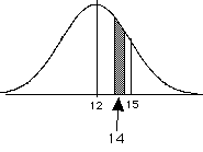m = pn = 12 s = sqroot (pqn) = sqr(48*.25*.75) = sqroot (9) = 3 from table X - m = 13.5 - 12.0 = 0.50 --> 0.3085 s 3 X - m = 14.5 - 12.0 = 0.83 --> 0.2033 s 3 so the area between the two z-scores is: 0.3085 - 0.2033 = 0.1052