Outline

Hypothesis testing framework
1-sample z-test
Using Excel for z-tests

Lab 15

Hypothesis testing continued & z-tests.

In our last lab we outlined steps involved in the inferential procedure of Hypothesis testing.

Hypothesis testing is an inferential procedure that uses sample data to evaluate the credibility of a hypothesis about a population.
Step 1: State the hypotheses and select a criteria for the decision Step 2: Collect a sample Step 3: Compute a test statistic Step 4: Compare the test statistic to a distribution to make an inference about the parameter and hence draw a conclusion about the sample

We covered in detail steps 1 & 2. In today's lab we'll focus on steps 3 & 4.

Step 3:Compute a test statistic

Included in our set of statistical tests are three different types of t-tests (we'll discuss these in the next few weeks). We strongly recommend that you download the t-test worksheet booklet and complete the summaries over the next few weeks (as we go through the different t-test labs).

Let's quickly recall the decision tree that we saw earlier in the semester.

Which test?

The diagram was designed to help you decide which design describes a research study. You will notice that the diagram you are viewing today has statistical tests added on the right side for each design. This diagram was developed to help you determine which test to use in different situations based on your answer to specific questions about the study you are looking at. The first question asks about the type of research question you are trying to answer. For the tests listed in the chart (and that we are discussing in this class), you are either looking at differences or relationships.

If you are looking for a relationship, you will either use the Pearson r correlation test or the Chi-square test ( we'll discuss these tests in later labs). You can also examine the linear regression line to determine the form of the realtionship. These tests are listed at the bottom of the diagram. The difference between the tests is what type of data you have. For interval-ratio data (numerical scores), use the Pearson r or Linear Regression. For nominal and ordinal data (data are frequency counts), use the Chi-square test.

The other tests in the chart look for differences between groups or conditions. The choice depends on several factors:

how many samples you have (i.e., how many different groups of subjects were tested)
for more than one group, whether the groups were matched in some way or were independent (different people that are not connected across the groups)
for one group only, how many scores each subject gave
whether or not σ is known

By answering these questions, the chart will lead you to the correct test.

Now, let's use the chart to figure out which test to use for different sets of data.

Use the chart to figure out which test to use for each study described below. Based on the information given, indicate:

(a) Whether a one-tailed test can be used or if a two-tailed test is more appropriate? (remember to use a one-tailed whenever you can find a directional alternative hypothesis to increase power)

(b) What are the null and alternative hypotheses?

(c) What is the appropriate statistical test to compute

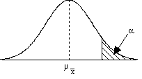
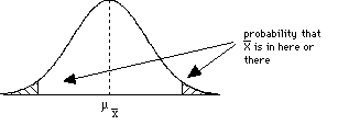
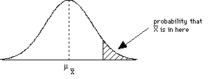
(1) People with agoraphobia are so filled with anxiety about being in public places that they seldom leave their homes. Knowing this is a difficult disorder to treat, a researcher tries a long-term treatment. A sample of individuals report how often they have ventured out of the house in the past month. Then they receive relaxation training and are introduced to trips away from the house at gradually increasing durations. After 2 months of treatment, subjects report the number of trips out of the house they made in the last 30 days. The researcher wants to determine if the number of trips out of the house has increased after the treatment.

(2) An experiment studied the effect of diet on blood pressure. Researchers randomly divided 54 healthy adults into two groups. One group received a calcium supplement. The other received a placebo. Blood pressure was measured at the end of one month of supplements or placebos.

(3) Suppose that during interpersonal social interactions (e.g., during business meetings or talking to causal acquaintances) people in the US maintain an average distance of μ=7 feet from other people. The distribution of distance scores is normal with a σ=1.5 feet. A researcher examines how the US compares in social interaction distance to social interaction distance for people in Italy. A random sample of 40 Italians is observed during interpersonal interactions. For this sample, the mean interaction distance is 4.5 feet. Do the Italians have closer social interactions than Americans do?

(4) The animal learning course in a university's psychology department requires that each student train a rat to perform certain behaviors. The student's grade is partially determined by the rat's performance. The instructor for the course has noticed that some students are very comfortable working with the rats and seem to be very successful training their rats. The instructor suspects that that these students may have previous experience with pets that gives them an advantage in the class. To test this hypothesis, the instructor gives the entire class a questionnaire at the beginning of the course. One question determines whether or not each student currently has a pet of any type at home. Based on the responses to this question, the instructor divides the class into two groups and compares the rats' learning scores for the two groups.

(5) A scientist investigated the authenticity of ESP abilities by asking subjects who claimed to have ESP abilities to predict the symbol that would appear on the back side of a succession of cards. Each card had a square, a circle, a star, or a triangle. Subjects were informed of this fact and were asked to predict what was on the back of each card as it was held up to them. Because the subjects could not see the backs of the cards, if they had no ESP abilities and simply guessed, they would get an average of .25 answers correct (so μ = .25). The scientist measured how many answers the subjects got correct out of 100 cards.

(6) A researcher is interested in how values taught to students by their parents influences their academic achievement. The parents of one group of students is asked to follow a program where they spend one hour per day discussing homework assignments with their child. In the other group, parents are given no program to follow. In order to control for genetic influences on academic achievement, the subjects in the study are identical twins raised apart (i.e., by different parents). One of the twins is randomly assigned to one group and the other twin is placed in the other group. Academic achievement is measured by GPA at the end of the first year of high school.

Step 4:Compare the test statistic to a distribution to make an inference about the parameter and draw a conclusion about the sample

After computing your test statistic, then you need to make a decision about your hypotheses. This will involve comparing your computed test statistic against a critical test statistic value that is based on your α (alpha-level), and whether you have a 1- or 2-tailed test (and for later tests, something called your degrees of freedom). Let's begin by look at pictures of distributions to try and connect this with what we've been talking about so far.

Consider the following sample mean distributions. The shaded regions correspond to critical regions that are defined by a critical test statistic determined by the alpha level (selected back in step 1) and whether the hypothesis is 1-tailed or 2-tailed.

α = prob of making a type I error

general alternative hypothesis

H₀: no difference
H₁: there is a difference

Two-tailed test
α = 0.05
so this is 0.025 in each tail 0.025 + 0.025 = 0.05

specific alternative hypothesis

₀

₁

One-tailed test
α = 0.05
so this is 0.05 in the tail

So how do we interpret these graphs?

₀

critical regions

The critical region is composed of extreme sample values that are very unlikely to be obtained if the null hypothesis is true. The size of the critical region is determined by the alpha level. Sample data that fall in the critical region will warrant the rejection of the null hypothesis.

Putting it all together

Now let's examine our first statistical test.

One-sample z test

Assumptions of the test (and most hypothesis testing)

Random sample

Independent observations

σ is known and is constant

the sampling distribution is relatively normal

Violations of any of these assumptions will severly compromise any conclusions that you make about the population based on your sample (basically, you need to use other kinds of inferential statistics that can deal with violations of various assumptions)

So far we've been discussing the logic of our Hypothesis Testing procedure. In this lab, we're going to cover one type of test statistic and put all the steps of hypothesis testing together. We're going to conduct hypothesis testing using the one-sample z-test. We've already covered the logic of how this works, but now we'll make it more formal as an inferential test statistic.

We can use the decision tree that we saw earlier in the semester (and opened earlier in the lab).

Find the string of decisions that lead to a 1-sample z-test.

The one-sample z-test is used to compare a single sample to a known population mean μ when we know:
(a) the distribution of sample means is normal
AND
(b) the population standard deviation σ is known.

Let's look at a complete example using our hypothesis testing steps:

Suppose we were interested in whether the number of hours students spend studying differs by class status (i.e., freshmen, sophomores, juniors, seniors). Specifically, we want to know if seniors spend more time studying than the average college student of any year. We know that the general population of college student in the US spends an average of 4 hours a day studying for their courses, with a σ = 1 hour. To answer our question, we'll ask a sample of 50 seniors how much time they spend studying per day.

In this study we are comparing a sample to a known population μ and σ. We also know that the distribution of sample means will be normal because our sample size is greater than 30. That means we can use our z-score procedure to conduct this test.

Step 1: State hypotheses and decision criterion.

For H_a: μ_seniors > 4
(because we are predicting that seniors study MORE)

For H₀: μ_seniors < 4
(because these are the other possibilities for the comparison)

Since our H_a is a directional hypothesis (we're only predicting an increase in study hours), we'll have a one-tailed test because we'll only need to consider the critical region above the null population mean.

We also need to set our alpha level for our decision criterion. We'll use α = .05. This is the highest probability of the null being true that we'll accept as evidence against it.

Step 2: Collect sample data

In this step, we actually collect our data. Suppose we asked the 50 seniors we selected for our sample how many hours a week they study and the average reported mean for the sample was = 4.4 hours. With our sample mean, we're ready to move on to Step 3 and calculate our z-score test statistic.

Step 3: Calculate test statistic

The first thing we need to do here is to calculate the standard error . We'll have:

= = 1/sq. root 50 = 1/7.07 = .14

Then we're ready to calculate z:

z = = (4.4 - 4) / .14 = 2.86

This is our test statistic. We'll need to know the probability of getting a sample mean this large or larger so we need to find z = 2.86 in the unit normal table.

Unit Normal table

We find that the probability of a sample mean this large or larger is .0021. Now it's time to do our last step to make our decision.

Step 4: Make a decision about H₀

We need to determine where our test statistic (z = 2.86) falls in the distribution by comparing it's p value with alpha. Is it in the critical region? In this case it is because it is lower than .05 so it would fall in the shaded region. This means there is less than a .0021 chance that we'd get a sample mean of 4.4 if seniors are the same as the general population. Since that's less than .05 (our decision criterion), that's low enough that we can decide that seniors come from a different population with a different mean than the general population of college students. This also means we have enough evidence to reject the H₀ hypothesis and accept H_a that seniors study more than the general population of college students. So our decision is:

Reject the null hypothesis and accept the alternative hypothesis.

Of course remember that there's still a chance (less than 5%) that we made a Type I error, but we're reasonably sure we made the right decision.

One last note about statistical significance: Remember from the last lab that the larger the sample size, the more likely we are to detect an effect that exists, because we're more likely to reject the null hypothesis. However, this also means that with large sample sizes, even if the effect is really small, we're more likely to reject the null and decide there's an effect. Therefore, in the case of very large samples, we may detect effects that lack practical significance because it is small enough to be not important. We must be careful that when we find statistical significance that our findings also have practical significance, meaning the effect of the treatment is important.

(7) Suppose we think that listening to classical music will affect the amount of time it takes a person to fall asleep so we conduct a study to test this idea.

(a) Suppose that the average person in the population falls asleep in 15 minutes (without listening to classical music) with σ = 6 min, state the null and alternative hypotheses for this study.

(b) Assume that the amount of time it takes people in the population to fall asleep is normally distributed. In the study we have a sample of people listen to classical music and then we measure how long it takes them to fall asleep. Suppose the sample of 36 people fall asleep in 12 minutes. What is the probability of obtaining a sample mean of 12 minutes or smaller? Assuming α = .05, is your calculated p value in the critical region (Hint: remember to consider two critical regions)?

(d) Assume now that in reality classical music does not affect how long it takes people to fall asleep. In this case, what kind of decision (correct, Type I error or Type II error) have you made in part (c)?

Ok, now try a couple more. For problems (8) - (9), write out each step of hypothesis testing.

(8) A psychologist examined the effect of chronic alcohol abuse on memory. In this study, a standardized memory test was used. Scores on this test for the general population form a normal distribution with μ = 50 and σ = 6. A sample of n = 22 alcohol abusers had a mean score of = 47. Is there evidence for memory impairment among alcoholics? Use α = .05 for a one-tailed test.

(9) On a vocational interest inventory that measures interest in several categories, a very large standardization group of adults (i.e., a population) has an average score of μ = 22 and σ = 4. Scores are normally distributed. A researcher would like to determine if scientists differ from the general population in terms of writing interests. A random sample of scientists is selected from the directory of a national science society. The scientists are given the inventory, and their test scores on the literary scale are as follows: 21, 20, 23, 28, 30, 24, 23, 19. Do scientists differ from the general population in their writing interests? Test at the .05 level of significance for two tails.

Using the z-test spreadsheet

Although you can calculate all of these things on your own, Dr. Joel Schneider has made this process easier with another spreadsheet that automates the z-test.

Download the z-test spreadsheet.

You have to enter the sample mean, population mean, population standard deviation, sample size, and α. You also have to specify which kind of test to perform (2-tailed or which direction the 1-tailed test goes). The standard error, observed z, critical z, and p-value are calculated. In addition, the decision to reject or retain the null hypothesis is printed. You can also look at the graph to see if the observed z falls in the critical region(s).

Always check the graph to see if makes sense because it is easy to enter the wrong numbers in the dark gray cells or forget to specify the right kind of test.

Here is an example that uses this spreadsheet program to find the solution.

Suppose that in the entire telemarketing sector, employees’ dissatisfaction with their jobs is μ = 40 and σ = 4 on a questionnaire. Low scores mean happier workers. High scores mean more dissatisfied workers. DirectXYZ is a firm that believes that its policies are significantly better at keeping its telemarketers happy on the job. At DirectXYZ, a sample of N = 25 employees randomly selected scored a sample mean of X¯ = 38.5 on the worker dissatisfaction questionnaire. Assume that α = 0.05.

If the correct numbers and options are entered into the spreadsheet, you can see a tiny red line in the green region at the left. This means that the observed z is in the critical region (i.e., it is more extreme than the critical z.) Thus, the null hypothesis should be rejected.

Here is how I would complete the type of questions in the lab:

In order to reject the null hypothesis, the observed z must be: ≤ −1.64
Observed z = −1.875
p = 0.0304
Reject or retain the Null hypothesis? Reject
State conclusion in everyday language: Telemarketers at DirectXYZ are, on average, less dissatisfied with their jobs than telemarketers at other firms.

Note: Had the data been different and the null hypothesis were retained, the conclusion in everyday language might have been: "There is no evidence that telemarketers at DirectXYZ are happier than comparable employees at other telemarketing firms."

Note: Had the 1-tailed hypothesis been in the other direction, the answer would have been “≥ 1.64.” Had the hypothesis been 2-tailed, the answer would have been “≤ −1.96 or ≥ 1.96.”

Note: Be careful about 1-tailed hypotheses! Sometimes you get an extreme result in the opposite direction of what you expect and you have to retain the null hypothesis, even though it looks like there was a large difference between the sample mean and the population mean.

You will probably have an easier time using the z-test spreadsheet described above, however I strongly suggest that you do the calculations yourself to make sure that you understand everything the underlying concepts and then check your answers using the spreadsheet.