A First Course for Students of Psychology and Education, 4th Edition. New York: West Publishing.
Correlation is a statistical technique that measures and describes the relationship between two variables.
-
Notice that this means that there must be at least two scores from each individual,
one for each of the two variables.
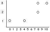
Consider the follwing example:
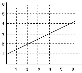
| Data Set | Scatterplot | |
Person	X	Y
    A	1	1
    B 	1	3
    C 	3	2
    D 	4	5
    E	6	4
    F	7	5
|
Y | 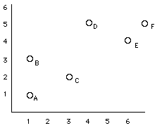 |
| X |
-
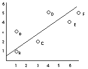
A correlation tells us about three characteristics about the relationship between X and Y
1) The direction of the relationship
positive correlation (a positive number) means that the two variables tend to move in the same direction. That is, as one gets larger, so does the other.
negative correlation (a negative number) means that the two variables tend to move in opposite directions. That is, as one gets larger, the other gets smaller.
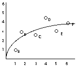
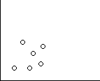
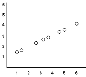
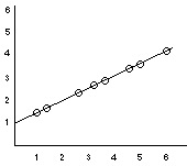
2) The form of the relationship
we will focus on linear correlations (straight lines), but there are also other forms that the relationship can take.
| linear (e.g., height and weight) | non-linear (e.g., age and height) |
 |
 |
-
3) The degree of the relationship
-
A correlation also measures the "strength" of the relationship between X and
Y. A correlation will have a value between -1 and +1. A correlation
of 0 means that there is no relationship. A +1 means that there is a
positive "perfect correlation" between two, and a -1 means that there
is a negative perfect correlation.
Why (and When) do we use correlations?
Prediction - if we know that two variables are strongly related, then we may be able to predict the value of one, based on the value of the other.
e.g., if you know that ultrasound measurements of a baby's head are positively correlated with birth weight, then you can make an educated guess of the baby's birth weight by measuring the baby's head from an ultrasound
Validity - if you develop a new test (TEST A) for X, and you want to know whether it is truely measuring X, then you can see if TEST A correlates with things that you already know correlate with X.
e.g., if you discover a new formula for predicting birth weight (imagine some magic formula that includes the height and weight of the mother and father combined), then this formula should also correlate with the ultrasound estimates of birthweight.
Reliability - if you use the same test twice on the same individuals, you can correlate the two sets of scores. If the test is reliable, then it should give similar results both times, giving you a high correlation
Theory Verification - many theories will predict that a relationship exists between different variables. So you can then go out, collect some data, and see if such a relationship exists.
Okay, so how do we quantify the idea of correlation? There are a number of different correlations, we will focus on the most common measure, the Pearson product-moment correlation.
	r    =   degree to which X and Y vary together     =       covariability of X and Y
		degree to which X and Y vary separately       variability of X and Y separately
-
That's what it means conceptually, but what exactly does that mean?
-
covary means that as X changes, Y also changes.
remember that a "perfect correlation" is r = 1.0 (or -1.0). This means that the number in the numerator equals the number in the denominator. On the bottom, we have two things, how much does X change and how much does Y change. On the top we have, how much to X and Y change together. If these three parts add up to the same thing, then we have and r = 1.0.
now let's consider how we actually compute r.
need to introduce a new concept: sum of products of deviations (SP)
-
this is the definitional formula
in other words, we figure out the average values for X and
Y. Then we figure out, for each point, how far away from
these means each point is, then multiply the X and Y
deviations, and then add them all up.
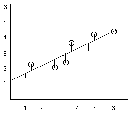
Consider the following:
X Y X- |
 |
|
So: SP = 14 |
-
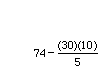
we can also compute SP with a computational formula:
X Y XY 0 1 0 10 3 30 4 1 4 8 2 16 8 3 24 30 10 74 |
SP = 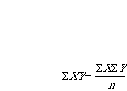
= = 74 - 60 = 14 |
Hopefully, SP reminds you of SS (Sum of Squares). The concepts are very similar. The basic difference is that with SS, we just had one variable (X), however with SP we have two variables (X & Y).
| Sum of Squares (SS) | Sum of products (SP) |
SS =  |
SP = |
SS = 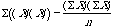 |
SP = |
-
Try to keep this in mind, it should help you remember SP.
Okay, now let's compute the pearson correlation (r).
-
This is what we know so far:
	r    = 	 degree to which X and Y vary together   =       covariability of X and Y
		degree to which X and Y vary separately     variability of X and Y separately
-
Let's expand on this using our new component SP
r = 
in other words, we've got SP on top, which is our measure of covariability of X and Y. On the bottom we've got our measure of variability of X alone and Y alone
so let's return to our example:
-
we've already got our SP, but we do need to figure out SSX & SSY
X Y X-Y-
(devX)(devY) (X-
-
r =
=  = 14/16 = +0.875
So there is a fairly strong positive correlation, as X goes up we can predict that Y will too.
-
1) The direction of the relationship - positive or negative
2) The form of the relationship - linear or non-linear
3) The degree of the relationship - the "strength" of the relationship
But there are some additional things that we need to consider.
-
4) Correlations describe a relationship between two variables, but
DOES NOT explain why the variables are related
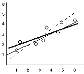
5) Correlations are greatly affected by the range of scores in the data
6) Extreme scores can have dramatic effects on correlations
7) When considering "how good" a relationship is, we really should consider r2, not just r.
Let's look at each point in a little more depth
4) Correlations describe a relationship between two variables, but DOES NOT explain why the variables are related
-
The basic underlying reason for this is that in a correlational
study, we, the experimenters, don't have control. That is,
we are not manipulating one (or more) variable(s) while
keeping everything else constant.
-
as a result, we can't make causal claims
e.g.,
a) Suppose that Dr. Steward finds that rates of spilled coffee and severity of plane turbulents are strongly positively correlated.
correlationally speaking, one might argue that spilling coffee causes turbulents
b) Suppose that Dr. Cranium finds a positive correlation between head size and digit span (describe digit span).
correlationally speaking, one might argue that people with bigger heads have bigger digit spans (instead of something like, head size and digit span increase with age)
c) Suppose the Dr. Ruth finds a positive correlation between the number of baby's born and the rate of stork sightings (I believe that such a correlation has been reported)
correlationally speaking, one might interpret this as support for the hypothesis that storks bring babies to home
-
We've already seen an example of this. Consider the
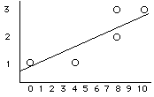
correlation between age and height.
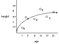
Suppose that in one study we look for a correlation between age and height, but we only test 0 to 10 yr olds. But in a second study we look for the same relationship but only test 25 to 25 yr olds. In the first case we will probably find a strong positive correlation, but in the later case we may find a near 0 correlation.
Which correlation is correct? Both are, if considered with respect to the range represented in the data. We should conclude that the strong positive correlation exists for a restricted range. That is, from years 0 to 10, there is a strong positive correlation between age and height. (note: a non-linear function is appropriate for this relationship)
-
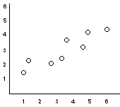
A single extreme score can really mess up a correlation.
 | 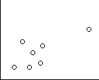 |
| r = -0.05 | r = +0.76 |
7) When considering "how good" a relationship is, we really should consider r2, not just r.
r2 is called the coefficient of determination
we'll talk more about this towards the end of this chapter. What it basically measures is how much of the variability in one variable can be determined by the other variable.
In other words, suppose that we find that the correlation (r) between height and weight is 0.76. We can use this information to predict a person's weight, if we know their height. But, notice that the correlation is not perfect, so we know that we may be off by a bit.
But we also know that we'll be close. The r2 for this relationship is (0.76)2 = .578. What we can conclude from this is that 57.8% of the variability in weight can be accounted for from the relationship that it has with height.
notice that if we do have a perfect correlation (r = ± 1.0), then r2 = 1.02 = 1.0. So 100% of the variance in Y can be accounted for by X.
 (pronounced "Y-hat")

 =
=  =
= 
 = .559